Understanding First-Order Ordinary Differential Equations: Geometric and Numerical Approaches

OK, let's get started. Now... I'm assuming that, A, you went recitation yesterday, B, that even if you didn't, you know how to separate variables, and you know how to construct simple models, solve physical problems with differential equations, and possibly even solve them.

So, you should have learned that either in high school, or 18.01 here, or... yeah. So, I'm going to start from that point, assume you know that. I'm not going to tell you what differential equations are, or what modeling is. If you still are uncertain about those things, the

book has a very long and good explanation of it. Just read that stuff. So, we are talking about first order ODEs. ODE: I'll only use three ... two acronyms. ODE is ordinary differential equations. I think all of MIT

knows that, whether they've been taking the course or not. So, we are talking about first-order ODEs. which in standard form, are written, you isolate the derivative of y with respect to, x, let's say, on the left-hand side, and on the right-hand side you write everything

else. You can't always do this very well, but for today, I'm going to assume that it has been done and it's doable. So, for example, some of the ones that will be considered either today or in the problem set are things like

oh... y' = x / y That's pretty simple. The problem set has y' = ...let's see... x - y^2.

And, it also has y' = y - x^2. There are others, too. Now, when you look at this, this, of course, you can solve by separating variables. So, this is solvable. This one is-- and neither of these can you

separate variables. And they look extremely similar. But they are extremely dissimilar. The most dissimilar about them is that this one is easily solvable. And you will learn, if you don't know already, next time next Friday how to solve this one

This one, which looks almost the same, is unsolvable in a certain sense. Namely, there are no elementary functions which you can write down, which will give a solution of that differential equation. So, right away, one confronts the most significant fact that

even for the simplest possible differential equations, those which only involve the first derivative, it's possible to write down extremely looking simple guys. I'll put this one up in blue to indicate that it's bad. Whoops, sorry, I mean, not really

bad, but recalcitrant. It's not solvable in the ordinary sense in which you think of an equation is solvable. And, since those equations are the rule rather than the exception, I'm going about this first day to not solving a single differential equation, but indicating

to you what you do when you meet a blue equation like that. What do you do with it? So, this first day is going to be devoted to geometric ways of looking at differential equations and numerical. At the very end, I'll talk a little bit about

numerical ways. And you'll work on both of those for the first problem set. So, what's our geometric view of differential equations? Well, it's something that's contrasted with

the usual procedures, by which you solve things and find elementary functions which solve them. I'll call that the analytic method. So, on the one hand, we have the analytic ideas, in which you write down explicitly the equation, y' = f(x,y).

And, you look for certain functions, which are called its solutions. Now, so there's the ODE. And, y1 of x, notice I don't use a separate letter. I don't use g or h or something like that for the solution because the letters multiply so quickly, that is, multiply in

the sense of rabbits, that after a while, if you keep using different letters for each new idea, you can't figure out what you're talking about. So, I'll use y1 means, it's a solution of this differential equation. Of course, the

differential equation has many solutions containing an arbitrary constant. So, we'll call this the solution. Now, the geometric view, the geometric guy that corresponds to this version

of writing the equation, is something called a direction field. And, the solution is, from the geometric point of view, something called an integral curve.

So, let me explain if you don't know what the direction field is. I know for some of you, I'm reviewing what you learned in high school. Those of you who had the BC syllabus in high school should know

these things. But, it never hurts to get a little more practice. And, in any event, I think the computer stuff that you will be doing on the problem set, a certain amount of it should be novel to you.

It was novel to me, so why not to you? So, what's a direction field? Well, the direction field is, you take the plane, and in each point of the plane-- of course, that's an impossibility. But, you pick some points of the plane. You draw what's called a little

line element. So, there is a point. It's a little line, and the only thing which distinguishes it outside of its position in the plane, so here's the point, (x,y), at which we are drawing this line element, is its slope. And, what is its slope? Its slope is to be f(x,y).

And now, You fill up the plane with these things until you're tired of putting then in. So, I'm going to get tired pretty quickly. So, I don't know, let's not make them all go the same way. That sort of seems cheating.

How about here? Here's a few randomly chosen line elements that I put in, and I putted the slopes at random since I didn't have any particular differential equation in mind. Now, the integral curve, so those are the line elements. The integral curve is a curve,

which goes through the plane, and at every point is tangent to the line element there. So, this is the integral curve. Hey, wait a minute, I thought tangents were the line element there didn't even touch it. Well, I can't fill up the plane with line elements.

Here, at this point, there was a line element, which I didn't bother drawing in. And, it was tangent to that. Same thing over here: if I drew the line element here, I would find that the curve had exactly the right slope there.

So, the point is the integral, what distinguishes the integral curve is that everywhere it has the direction, that's the way I'll indicate that it's tangent, has the direction of the field everywhere at all points on the curve, of course, where it doesn't go. It doesn't

have any mission to fulfill. Now, I say that this integral curve is the graph of the solution to the differential equation. In other words, writing down analytically the differential equation is the same geometrically as drawing this direction field, and solving analytically

for a solution of the differential equation is the same thing as geometrically drawing an integral curve. So, what am I saying? I say that an integral curve,

all right, let me write it this way. I'll make a little theorem out of it, that y1(x) is a solution to the differential equation if, and only if,

the graph, the curve associated with this, the graph of y1 of x is an integral curve. Integral curve of what? Well, of the direction field associated with that equation. But there isn't quite enough room to write that on the board. But, you could put it in your notes, if you

take notes. So, this is the relation between the two, the integral curves of the graphs or solutions. Now, why is that so? Well, in fact, all I have to do to prove this, if you can call

it a proof at all, is simply to translate what each side really means. What does it really mean to say that a given function is a solution to the differential equation? Well, it means that if you plug it into the differential equation, it satisfies it. Okay, what is that?

So, how do I plug it into the differential equation and check that it satisfies it? Well, doing it in the abstract, I first calculate its derivative. And then, how will it look after I plugged it into the differential equation? Well, I don't do anything to the x, but wherever

I see y, I plug in this particular function. So, in notation, that would be written this way. So, for this to be a solution means this, that that equation is satisfied. Okay, what

does it mean for the graph to be an integral curve? Well, it means that at each point, the slope of this curve, it means that the slope of y1 of x should be, at each point, (x1,y1). It should be equal to the slope of the direction field at that point.

And then, what is the slope of the direction field at that point? Well, it is f of that particular, well, at the point, (x,y1). If you like, you can put a subscript, one, on there, send a one here or a zero there, to indicate that you mean a particular point.

But, it looks better if you don't. But, there's some possibility of confusion. I admit to that. So, the slope of the direction field, what is that slope? Well, by the way, I calculated the direction field. Its slope at the point was to be x, whatever the value of x was,

and whatever the value of y1(x) was, substituted into the right-hand side of the equation. So, what the slope of this function of that curve of the graph should be equal to the slope of the direction field. Now, what does this say?

Well, what's the slope of y1(x)? That's y1'(x). That's from the first day of 18.01, calculus. What's the slope of the direction field? This? Well, it's this. And, that's with the right hand side. So, saying these two guys are the same or equal, is exactly, analytically, the

same as saying these two guys are equal. So, in other words, the proof consists of, what does this really mean? What does this really mean? And after you see what both really mean, you say, yeah, they're the same.

So, I don't how to write that. It's okay: same, same, how's that? This is the same as that. Okay, well, this leaves us the interesting question of how do you draw a direction from the, well, this being 2003, mostly computers draw them for you. Nonetheless, you do have

to know a certain amount. I've given you a couple of exercises where you have to draw the direction field yourself. This is so you get a feeling for it, and also because humans don't draw direction fields the same way computers do. So, let's first of all, how did computers

do it? They are very stupid. There's no problem. Since they go very fast and have unlimited amounts of energy to waste, the computer method is the naive one. You pick the point. You pick a point, and generally, they are usually

equally spaced. You determine some spacing, that one: blah, blah, blah, blah, blah, blah, blah, equally spaced. And, at each point, it computes f(x, y) at the point, finds, meets, and computes the value of f of (x, y), that function, and the next thing is, on the screen,

it draws, at (x, y), the little line element having slope f(x, y). In other words, it does what the differential equation tells it to do. And the only thing that it does is you can, if you are telling the thing to draw the direction

field, about the only option you have is telling what the spacing should be, and sometimes people don't like to see a whole line. They only like to see a little bit of a half line. And, you can sometimes tell, according to the program, tell the computer how long you

want that line to be, if you want it teeny or a little bigger. Once in awhile you want you want it narrower on it, but not right now. Okay, that's what a computer does. What does a human do? This is what it means to be human.

You use your intelligence. From a human point of view, this stuff has been done in the wrong order. And the reason it's been done in the wrong order: because for each new point, it requires a recalculation of f(x, y). That is horrible. The computer doesn't mind, but

a human does. So, for a human, the way to do it is not to begin by picking the point, but to begin by picking the slope that you would like to see. So, you begin by taking the slope. Let's call it the value of the slope, C. So, you pick a number. C is two.

I want to see where are all the points in the plane where the slope of that line element would be two? Well, they will satisfy an equation. The equation is f(x,y) = C, in general. So, what you do is plot this, plot the equation,

plot this equation. Notice, it's not the differential equation. You can't exactly plot a differential equation. It's a curve, an ordinary curve. But which curve will depend; it's, in fact, from the 18.02 point of view, the level curve of C, sorry, it's a level curve of f of (x,

y), the function f of x and y corresponding to the level of value C But we are not going to call it that because this is not 18.02. Instead, we're going to call it an isocline. And then, you plot, well, you've done it. So, you've got this isocline,

except I'm going to use a solution curve, solid lines, only for integral curves. When we do plot isoclines, to indicate that they are not solutions, we'll use dashed lines for doing them. One of the computer things does and the other one doesn't. But they use

different colors, also. There are different ways of telling you what's an isocline and what's the solution curve. So, and what do you do? So, these are all the points where the slope is going to be C.

And now, what you do is draw in as many as you want of line elements having slope C. Notice how efficient that is. If you want 50 million of them and have the time, draw in 50 million. If two or three are enough, draw in two or three. You will be looking

at the picture. You will see what the curve looks like, and that will give you your judgment as to how you are to do that. So, in general, a picture drawn that way, so let's say, an isocline corresponding to C equals zero.

The line elements, and I think for an isocline, for the purposes of this lecture, it would be a good idea to put isoclines. Okay, so I'm going to put solution curves in pink, or whatever this color is, and isoclines are going to be in orange, I guess. So, isocline,

represented by a dashed line, and now you will put in the line elements of, we'll need lots of chalk for that. So, I'll use white chalk. Y horizontal? Because according to this the slope is supposed to be zero there. And at

the same way, how about an isocline where the slope is negative one? Let's suppose here C is equal to negative one. Okay, then it will look like this. These are supposed to be lines of slope negative one. Don't shoot me if they are not. So, that's the principle.

So, this is how you will fill up the plane to draw a direction field: by plotting the isoclines first. And then, once you have the isoclines there, you will have line elements. And you can draw

a direction field. Okay, so, for the next few minutes, I'd like to work a couple of examples for you to show how this works out in practice. So, the first equation is going

to be y' = -x / y. Okay, first thing, what are the isoclines? Well, the isoclines the isoclines are going to be y.

Well, -x / y = C. Maybe I better make two steps out of this. Minus x over y is equal to C. But, of course, nobody draws a curve in that form. You'll want it in the form y = -1 / C * x. So, there's our isocline. Why don't I put that up in orange since it's going

to be, that's the color I'll draw it in. In other words, for different values of C, now this thing is aligned. It's aligned, in fact, through the origin. This looks pretty simple. Okay, so here's our plane. The isoclines are going to be lines through the origin. And

now, let's put them in, suppose, for example, C is equal to one. Well, if C is equal to one, then it's the line, y equals minus x. So, this is the isocline. I'll put, down here, C equals minus one. And,

and along it, the no, something's wrong. I'm sorry?

C is one, not negative one, right, thanks. Thanks. So, C equals one. So, it should be little line segments of slope one will be the line elements, things of slope one. OK, now how about C equals negative one?

If C equals negative one, then it's the line, y = x. And so, that's the isocline. Notice, still dash because these are isoclines. Here, C is negative one. And so, the slope elements look like this. Notice, they are perpendicular. Now, notice that they are always going to

be perpendicular to the line because the slope of this line is minus one over C. But, the slope of the line element is going to be C. Those numbers, minus one over C and C, are negative reciprocals. And, you know that two lines whose slopes are negative reciprocals

are perpendicular. So, the line elements are going to be perpendicular to these. And therefore, I hardly even have to bother calculating, doing any more calculation. Here's going to be a, well, how about this one?

Here's a controversial isocline. Is that an isocline? Well, wait a minute. That doesn't correspond to anything looking like this. Ah-ha, but it would if I put C multiplied through by C. And then, it would correspond to C being zero. In other words, don't write

it like this. Multiply through by C. It will read C y = - x. And then, when C is zero, I have x equals zero, which is exactly the y-axis. So, that really is included. How about the x-axis? Well, the x-axis is not included.

However, most people include it anyway. This is very common to be a sort of sloppy and bending the edges of corners a little bit, and hoping nobody will notice. We'll say that corresponds to C equals infinity. I hope nobody wants to fight about that. If you do, go fight

with somebody else. So, if C is infinity, that means the little line segment should have infinite slope, and by common consent, that means it should be vertical. And so, we can even count this as sort of an isocline. And, I'll make the dashes smaller, indicate

it has a lower status than the others. And, I'll put this in, do this weaselly thing of putting it in quotation marks to indicate that I'm not responsible for it. Okay, now, we now have to put it the integral curves. Well, nothing could be easier. I'm

looking for curves which are everywhere perpendicular to these rays. Well, you know from geometry that those are circles. So, the integral curves are circles. And, it's an elementary exercise,

which I would not deprive you of the pleasure of. Solve the ODE by separation of variables. In other words, we've gotten the, so the circles are ones with a center at the origin, of course, equal some constant. I'll call it C1, so it's not confused with this C. They look like that,

and now you should solve this by separating variables, and just confirm that the solutions are, in fact, those circles. One interesting thing, and so I confirm this, I won't do it because I want to do geometric

and numerical things today. So, if you solve it by separating variables, one interesting thing to note is that if I write the solution as y = y1(x), well, it'll look something like the sqrt (C1 - x^2). We'll make the x squared because that's the way people usually put the radius.

Minus x squared. And so, a solution, a typical solution looks like this. Well, what's the solution over here? Well, that one solution will be goes from here to here. If you like, it has a negative

side to it. So, I'll make, let's say, plus. There's another solution, which has a negative value. But let's use the one with the positive value of the square root. My point is this, that that solution, the domain of that solution, really only goes from here to here. It's not

the whole x-axis. It's just a limited piece of the x-axis where that solution is defined. There's no way of extending it further. And, there's no way of predicting, by looking at the differential equation, that a typical solution was going to have a limited domain

like that. In other words, you could find a solution, but how far out is it going to go? Sometimes, it's impossible to tell, except by either finding it explicitly, or by asking a computer

to draw a picture of it, and seeing if that gives you some insight. It's one of the many difficulties in handling differential equations. You don't know what the domain of a solution is going to be until you've actually calculated it.

Now, a slightly more complicated example is going to be, let's see, y' = 1 + x - y. It's not a lot more complicated, and as a computer exercise, you will work with, still, more complicated ones. But here, the isoclines would be what? Well, I set that equal to C.

Can you do the algebra in your head? An isocline will have the equation: this equals C. So, I'm going to put the y on the right hand side, and that C on the left hand side. So, it will have the equation y = 1 + x - C, or a nicer way to write it would be y = x + 1 - C. I

guess it really doesn't matter. So there's the equation of the isocline. Let's quickly draw the direction field. And notice, by the way, it's a simple equation, but you cannot separate variables. So, I will not,

today at any rate, be able to check the answer. I will not be able to get an analytic answer. All we'll be able to do now is get a geometric answer. But notice how quickly, relatively quickly, one can get it. So, I'm feeling for how the solutions behave to this equation.

All right, let's see, what should we plot first? I like C equals one, no, don't do C equals one. Let's do C equals zero, first. C equals zero. That's the line. y = x + 1. Okay, let me run and get that chalk.

So, I'll isoclines are in orange. If so, when C equals zero, y equals x plus one. So, let's say it's this curve. C equals zero.

How about C equals negative one? Then it's y = x + 2. It's this curve. Well, let's label it down here.

So, this is C equals negative one. C equals negative two would be y equals x, no, what am I doing? C equals negative one is y = x + 2. That's right. Well, how about the other side? If C equals plus one, well, then it's going to go through the origin.

It looks like a little more room down here. How about, so if this is going to be C equals one, then I sort of get the idea. C equals two will look like this. They're all going to be parallel lines because all that's changing is the y-intercept, as I do this thing. So, here, it's C equals

two. That's probably enough. All right, let's put it in the line elements. All right, C equals negative one. These will be perpendicular. C equals zero, like this. C equals one. Oh, this is interesting. I can't even draw in the line elements because they

seem to coincide with the curve itself, with the line itself. They write y along the line, and that makes it hard to draw them in. How about C equals two? Well, here, the line elements will be slanty. They'll have slope two, so a pretty slanty up. And, I can see if a C

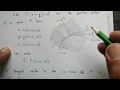
equals three in the same way. There are going to be even more slantier up. And here, they're going to be even more slanty down. This is not very scientific terminology or mathematical, but you get the idea. Okay, so there's our quick version of the direction field. All

we have to do is put in some integral curves now. Well, it looks like it's doing this. It gets less slanty here. It levels out, has slope zero. And now, in this part of the plain, the slope seems to be rising. So, it must do something

like that. This guy must do something like this. I'm a little doubtful of what I should be doing here. Or, how about going from the other side? Well, it rises, gets a little, should it cross this? What should I do? Well, there's one integral curve, which is easy

to see. It's this one. This line is both an isocline and an integral curve. It's everything, except drawable, [LAUGHTER] so, you understand this is the same line. It's both orange and pink at the same time. But I don't know what combination color that

would make. It doesn't look like a line, but be sympathetic. Now, the question is, what's happening in this corridor? In the corridor, that's not a mathematical word either, between the isoclines for, well, what are they? They are the isoclines for C equals two, and C

equals zero. How does that corridor look? Well: something like this. Over here, the lines all look like that. And here, they all look like this.

The slope is two. And, a hapless solution gets in there. What's it to do? Well, do you see that if a solution gets in that corridor, an integral curve gets in that corridor, no escape is possible. It's like a lobster trap. The lobster can walk in. But it cannot walk

out because things are always going in. How could it escape? Well, it would have to double back, somehow, and remember, to escape, it has to be, to escape on the left side, it must be going horizontally.

But, how could it do that without doubling back first and having the wrong slope? The slope of everything in this corridor is positive, and to double back and escape, it would at some point have to have negative slope. It can't do that. Well, could it escape on the

right-hand side? No, because at the moment when it wants to cross, it will have to have a slope less than this line. But all these spiky guys are pointing; it can't escape that way either. So, no escape is possible. It has to continue on, there. But, more than

that is true. So, a solution can't escape. Once it's in there, it can't escape. It's like, what do they call those plants, I forget, pitcher plants. You know, all their hairs are going down. So, it looks like that. And so,

the poor little insect falls in. They could climb up the walls except that all the hairs are going the wrong direction, and it can't get over them. Well, let's think of it that way: this poor trap solution. So, it does what it has to do. Now, there's more to it

than that. Because there are two principles involved here that you should know, that help a lot in drawing these pictures. Principle number one is that two integral curves cannot cross at an angle. Two integral curves can't cross, I mean, by crossing at an angle like

that. I'll indicate what I mean by a picture like that. Now, why not? This is an important principle. Let's put that up in the white box. They can't cross because if two integral curves, are trying to cross, well, one will look like

this. It's an integral curve because it has this slope. And, the other integral curve has this slope. And now, they fight with each other. What is the true slope at that point? Well, the direction field only allows you to have one slope. If there's a line element

at that point, it has a definite slope. And therefore, it cannot have both the slope and that one. It's as simple as that. So, the reason is you can't have two slopes. The direction field doesn't allow it. Well, that's a big, big help because if I know, here's an integral

curve, and if I know that none of these other pink integral curves are allowed to cross it, how else can I do it? Well, they can't escape. They can't cross. It's sort of clear that they must get closer

and closer to it. You know, I'd have to work a little to justify that. But I think that nobody would have any doubt of it who did a little experimentation. In other words, all these curves joined that little tube and get closer and closer to this line, y = x.

And there, without solving the differential equation, it's clear that all of these solutions, how do they behave? As x goes to infinity, they become asymptotic to, they become closer and closer to the solution, x. Is x a solution? Yeah, because y equals x is an integral curve.

Is x a solution? Yeah, because if I plug in y equals x, I get what? On the right-hand side, I get one. And on the left-hand side, I get one. One equals one. So, this is a solution. Let's indicate that it's a solution. So, analytically, we've discovered an analytic solution to the

differential equation, namely, Y equals X, just by this geometric process. Now, there's one more principle like that, which is less obvious. But you do have to know it. So, you are not allowed to cross. That's clear. But it's much, much, much, much, much less obvious

that two integral curves cannot touch. That is, they cannot even be tangent. Two integral curves cannot be tangent. I'll indicate that by the word touch, which is what a lot of people say. In other words,

if this is illegal, so is this. Can't have it. You know, without that for example, it might

be, I might feel that there would be nothing in this to prevent those curves from joining. Why couldn't these pink curves join the line, y equals x? You know, it's a solution. They just pitch a ride, as it were. The answer is they cannot do that because they have to

just get asymptotic to it, ever, ever closer. They can't join y equals x because at the point where they join, you have that situation. Now, why can't you to have this? That's much more sophisticated than this, and the reason

is because of something called the Existence and Uniqueness Theorem, Existence and Uniqueness Theorem which says

which says which says that there is through a point, (x0, y0), that y prime equals y' = f(x, y) has only one, and only one solution. One has one solution.

In mathematics speak, that means at least one solution. It doesn't mean it has just one solution. That's mathematical convention. It has one solution, at least one solution. But, the killer is, only one solution.

That's what you have to say in mathematics if you want just one, one, and only one solution through the point (x0, y0). So, the fact that it has one, that is the existence part. The fact that it has only one is the uniqueness part of the theorem. Now, like all good mathematical

theorems, this one does have hypotheses. So, this is not going to be a course, I warn you, those of you who are theoretically inclined, very rich in hypotheses. But, hypotheses for those one or that f(x, y) should be a continuous function. Now, like polynomial, signs, should

be continuous near, in the vicinity of that point. That guarantees existence, and what guarantees uniqueness is the hypothesis that you would not guess by yourself. Neither would I. What guarantees the uniqueness is that also, it's

partial derivative with respect to y should be continuous, should be continuous near (x0, y0). Well,

I have to make a decision. I don't have time to talk about Euler's method. Let me refer you to the, there's one page of notes, and I couldn't do any more than just repeat what's on those notes. So, I'll trust you to read that.

And instead, let me give you an example which will solidify these things in your mind a little bit. I think that's a better course. The example is not in your notes, and therefore, remember, you heard it here first. Okay, so what's the example? It's...

So, there's our differential equation. Now, let's just solve it by separating variables. dy. Can you do it in your head? dy

over dx, put all the y's on the left. It will look like dy / (1 - y). Put all the dx's on the left. So, the dx here goes on the right, rather. That will be dx. And then, the x goes down into the denominator. So now, it looks like that.

And, if I integrate both sides, I get the log of one minus y, I guess, maybe with a, I never bothered with that, but you can. It should be absolute values. All right, put an absolute value, plus a constant. And now, if I exponentiate both sides, the constant

is positive. So, this is going to look like y. (1 - y) = x. And, the constant will be e^C1. And, I'll just make that a new constant, Cx. And now, by letting C be negative, that's why you can get rid of the absolute values, if you allow C to have negative values as

well as positive values. Let's write this in a more human form. So, y = 1 - Cx. Good, all right, let's just plot those. So, these are the solutions. It's a pretty easy equation, pretty easy solution method, just separation of variables. What

do they look like? Well, these are all lines whose intercept is at one. And, they have any slope whatsoever. So, these are the lines that look like that. Okay, now let me ask, existence and uniqueness. Existence: through which points of the plane does the solution

go? Answer: through every point of the plane, through any point here, I can find one and only one of those lines, except for these stupid guys here on the stalk of the flower. Here, for each of these points, there is no existence. There is no solution to this differential

equation, which goes through any of these wiggly points on the y-axis, with one exception. This point is oversupplied. At this point, it's not existence that fails. It's uniqueness that fails: no uniqueness. There are lots of things which go through here. Now, is that

a violation of the existence and uniqueness theorem? It cannot be a violation because the theorem has no exceptions. Otherwise, it wouldn't be a theorem. So, let's take a look. What's wrong? We thought we solved it modulo, putting the absolute value signs on

the log. What's wrong? The answer: what's wrong is to use the theorem you must write the differential equation in standard form, in the green form I gave you. Let's write the differential equation the way we were supposed to. It says dy / dx = (1 - y) / x.

And now, I see, the right-hand side is not continuous, in fact, not even defined when x equals zero, when along the y-axis. And therefore, the existence and uniqueness is not guaranteed along the line, x equals zero of the y-axis. And, in fact, we see that it

failed. Now, as a practical matter, it's the way existence and uniqueness fails in all ordinary life work with differential equations is not through sophisticated examples that mathematicians can construct.

But normally, because f(x, y) will fail to be defined somewhere, and those will be the bad points. Thanks.